RAG

docs.scrimba.com

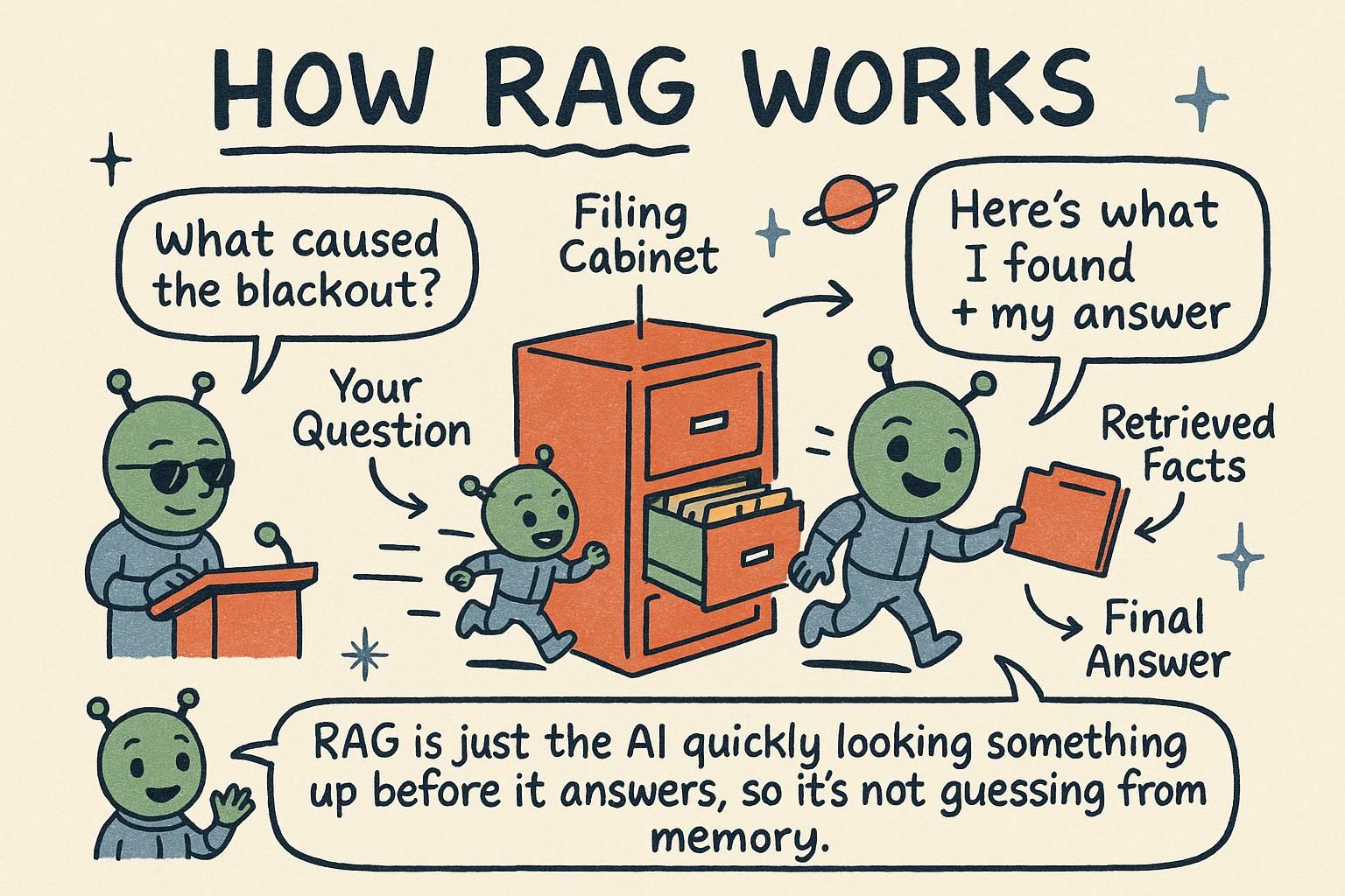
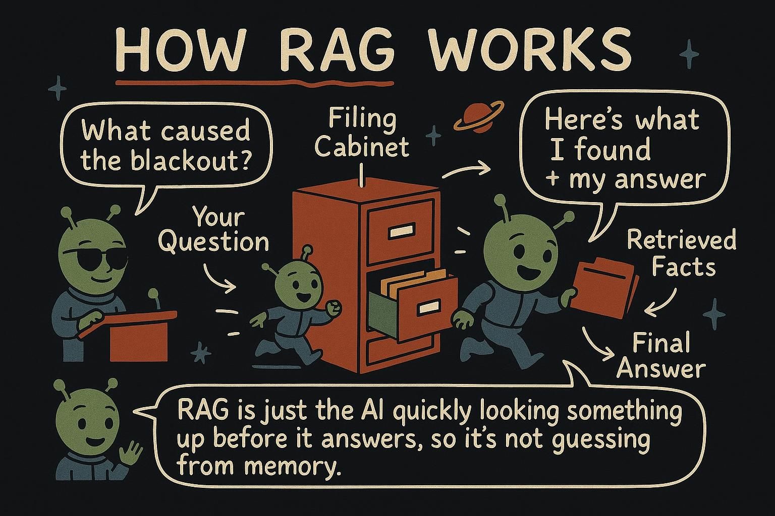
First, the name. RAG is short for retrieval-augmented generation: you fetch the relevant text yourself and hand it to the model at the moment of the question, so it answers from facts you supplied instead of from frozen memory. This chapter is how that fetch-then-answer loop works and where it goes wrong.

The retrieve-then-generate pattern

A model does not know your company's help docs, your product details, or anything that happened after it was trained. Ask it about them and it will either admit it cannot help or, worse, make something up that sounds right. RAG fixes this by handing the model the relevant text at the moment of the question.

The idea comes together once you have embeddings, the trick that turns text into vectors you can compare by closeness (cosine similarity measures how close two vectors point). Retrieval-augmented generation is two steps bolted onto a normal model call:

1. Retrieve. Take the user's question, search your documents for the most relevant pieces, and collect the top matches.
2. Generate. Put those pieces into the prompt as context, then ask the model to answer the question using only that context.

The model's general language ability does the writing; your retrieved text supplies the facts. You get fluent answers that are grounded in your content and can stay current, because you control what goes in.

It helps to see why this works so well, in terms of the prediction loop. Without RAG, you are asking the model to recall a fact from the patterns frozen into its parameters, which it may not have, leading to a confident guess. With RAG, the fact is sitting right there in the context, so the model's job changes from "remember this" to "read what is in front of you and answer from it". Retrieval moves the work from memory to reading. The clean picture is an exam: a closed-book exam invites guessing, while RAG turns it into an open-book exam where the relevant page is open on the desk.

JunoThe retrieve-then-generate pattern RAG adds two steps to a normal model call: retrieve the documents most relevant to the question, then generate an answer using them as context. The model supplies the language, your retrieved text supplies the facts. This lets it answer from your content instead of from memory, which is what stops it inventing answers. Took me a while to trust it, but an open-book model really does guess less than a closed-book one.

A model does not carry your help docs, your product details, or anything after its training cutoff. Ask anyway and you get a refusal or an invented answer that reads fine. Retrieval-augmented generation closes that gap by fetching relevant text and placing it in the prompt at request time, so the model reads the fact instead of recalling it. The mechanism rests on embeddings, where each piece of text becomes a vector and similarity is the distance between vectors (cosine similarity, the cosine of the angle between them).

The loop is two steps:

1. Retrieve. Embed the question into the same vector space as your documents, then pull the closest chunks by similarity.
2. Generate. Concatenate those chunks into the prompt as context, and instruct the model to answer only from them.

The retrieval step has a dial you set called top-k: how many of the closest chunks you actually keep. k is a balance. Too small and you miss the chunk that held the answer, so the model has nothing to work from. Too large and you pad the context with loosely related text, which dilutes the signal, raises cost, and makes the lost-in-the-middle problem worse. A k of 3 to 5 is a reasonable place to start, and you tune it against real questions.

Here is the move: structure the index as a list of records, each holding the chunk text and its precomputed vector, and structure the prompt so the retrieved context sits in a clearly delimited block above the question. The model's language ability writes; your retrieved text decides what is true.

def retrieve(question, index, k=4):
    query_vector = embed(question)
    scored = [
        {"text": item["text"], "score": cosine_similarity(query_vector, item["vector"])}
        for item in index
    ]
    return sorted(scored, key=lambda x: x["score"], reverse=True)[:k]

JunoThe retrieve-then-generate pattern RAG is retrieve then generate: embed the question, pull the closest chunks, drop them in the prompt, and answer from them. The dial that matters here is top-k, the number of chunks you keep: too few and you miss the answer, too many and you bury it in noise and pay for the privilege. Start around 3 to 5 and tune against real questions, not vibes.

A model does not hold your private corpus or anything past its cutoff, and it will not tell you which it is; it answers in the same confident tone either way. Retrieval-augmented generation is the pattern of fetching relevant text at request time and grounding the answer in it, so correctness rides on a source you control rather than on parametric recall. It runs on embeddings: text mapped to vectors, ranked by cosine similarity (the cosine of the angle between two vectors, so closeness of meaning regardless of length).

The two-step framing, retrieve then generate, is correct but hides where the work is. Retrieval is a search problem wearing a generation hat, and the quality of the whole system is set there, not in the model call. So treat retrieve-then-generate as retrieve-rank-then-generate from the start, because the naive version, embed the query, take the nearest k, paste them in, breaks on the failure modes the lower tiers have not met yet: exact-match misses, near-duplicate chunks crowding out coverage, and stale text answering confidently.

The first habit worth wiring in early is that this is a measurable system, not a vibe. Hold out a set of real questions with the chunks that should answer them, then track recall@k: of the chunks that should have been retrieved, the fraction that landed in your top k. Recall@k is your ceiling. If the right chunk is not in context, no amount of prompt craft recovers it, and the generate step cannot answer what retrieval never handed it. Everything downstream is bounded by this number, so it is the first thing to measure and the first thing to move.

def retrieve(question, index, k=8):
    query_vector = embed(question)
    scored = [
        {"text": it["text"], "score": cosine_similarity(query_vector, it["vector"]), "meta": it["meta"]}
        for it in index
    ]
    # over-fetch here, then re-rank down to a smaller final set (see below)
    return sorted(scored, key=lambda x: x["score"], reverse=True)[:k]

JunoThe retrieve-then-generate pattern RAG is a search problem wearing a generation hat: the quality is set in retrieval, not the model call, so the naive embed-take-k-paste version will let you down on exact matches and stale text. The number that bounds everything is recall@k, the fraction of the chunks that should have been retrieved that actually made your top k. If the right chunk never lands in context, no prompt saves you. Measure that before you tune anything else, or you are polishing the wrong end.

Chunking

You do not embed whole documents. You split them into smaller chunks first, a paragraph or a few sentences each, and embed those. Two reasons. First, retrieval gets more precise: you pull the one relevant paragraph instead of a whole 40-page manual. Second, chunks fit the context window, where a giant document might not.

# a small chunker: split on paragraphs
def chunk(text):
    return [c.strip() for c in text.split("\n\n") if c.strip()]

Chunk size is a balance, and the reason traces back to embeddings. Each chunk is turned into a single vector that summarises its whole meaning. Make a chunk too large and it covers several topics, so its one vector is a muddy average of all of them that matches no specific question well. Make it too small and it loses the surrounding meaning it needed to make sense, so the vector points at a fragment. Paragraph-sized chunks each hold one coherent idea. You adjust from there based on how your retrieval performs.

JunoChunking Before embedding, split documents into smaller chunks, roughly paragraph-sized, and embed those. Smaller chunks make retrieval more precise and fit the context window better. Chunk size is a balance: too large is fuzzy and wasteful, too small loses the surrounding meaning. When my answers came back vague, the chunks were almost always too big.

You embed chunks, not whole documents, because each chunk becomes one vector that has to summarise its whole meaning. Split a document into paragraph-sized pieces and embed each. Too large a chunk averages several topics into a vector that matches nothing sharply; too small a chunk loses the context that made it meaningful.

So treat chunk size as a tuning dial, not a fixed rule. A chunk of a few hundred tokens tends to hold one idea cleanly. The dial interacts with top-k: bigger chunks mean fewer of them fit your context budget, so you carry less coverage per request. Smaller chunks raise precision but need a larger k to reassemble an idea that spans them.

The second dial is overlap: let consecutive chunks share a slice of text at their boundaries, say 10 to 20 percent. Without overlap, a sentence that answers the question can land split across a boundary, half in one chunk and half in the next, so neither chunk retrieves well. Overlap costs you some duplication and a few more vectors, and it buys back the answers that boundaries would otherwise cut in two.

def chunk(text, size=800, overlap=120):
    # size and overlap in characters here; budget in tokens for real systems
    out, start = [], 0
    while start < len(text):
        out.append(text[start:start + size])
        start += size - overlap
    return out

JunoChunking Chunk size and overlap are tuning dials, not settings you get right once. Aim for chunks that hold one idea, a few hundred tokens, and remember the dial trades against top-k: bigger chunks, fewer fit. Add 10 to 20 percent overlap so an answer that straddles a boundary still lives whole inside at least one chunk. Boundaries are where retrieval quietly loses answers.

Chunking is where retrieval recall is won or lost before a single query runs. Each chunk becomes one vector that has to stand in for its entire meaning, so the split decides what is findable. Paragraph or section boundaries beat fixed character windows when the document has structure, because a vector over one coherent section is a cleaner query target than a vector over half of two sections.

Chunk size and overlap are coupled to your whole budget, not free parameters. Size trades against top-k against the context window: large chunks carry more context each but fewer fit, so coverage drops; small chunks raise precision but fragment ideas and need a higher k to reassemble, which costs tokens and reintroduces lost-in-the-middle. Overlap of roughly 10 to 20 percent rescues answers that straddle a boundary, at the cost of duplication in your index. The duplication has a downstream bite: near-identical overlapping chunks can fill several of your top-k slots with the same content, starving coverage. That is one of the reasons re-ranking and de-duplication earn their place later.

The cost most people skip until it hurts: chunking strategy is baked into your index, so changing it means re-embedding and re-indexing the entire corpus. That is real compute, real money, and a migration window where old and new vectors should not be mixed. Decide chunk size against your actual documents and queries early, measure recall@k on a held-out set, and treat a re-chunk as a deliberate re-index, not a config tweak you ship on a Friday.

JunoChunking Chunk on structure where you have it, because each chunk is one vector standing in for its whole meaning, and size trades against top-k against the window all at once. Overlap of 10 to 20 percent saves boundary-straddling answers but breeds near-duplicates that crowd your top-k, which is part of why re-ranking exists. And remember the chunking choice is baked into the index: changing it is a full re-embed and re-index, real cost and a migration, not a config flip.

Where vectors live

For a handful of chunks, you can keep the vectors in memory and compare them with the cosine-similarity function from the embeddings chapter, which is what the example later does. For thousands or millions of chunks, that gets slow, and you reach for a vector store: a database built to find the nearest vectors quickly at scale.

You do not need one to learn RAG, and you do not need to pick one now. Several exist as hosted services and libraries; the concept is what matters: somewhere to store embeddings and search them fast. Start in memory, move to a store when the collection outgrows it.

JunoWhere vectors live For a few chunks, keep vectors in memory and compare them directly. For large collections, a vector store is a database that finds nearest vectors quickly at scale. You do not need one to learn RAG: start in memory and move to a vector store when the collection outgrows it. No need to shop for a database on day one.

For a few hundred chunks, vectors live in memory and you score every one against the query. That is a linear scan: fine at small scale, slow once the collection runs to thousands or millions, because you compare against every vector on every query. At that point you move to a vector store, a database that indexes vectors for fast nearest-neighbor search.

The asymmetry worth holding onto is embed-once versus embed-per-query. You embed and index every document chunk exactly once, ahead of time, and that work is reused for every future question. You embed the query once per request, at request time, and that is the only embedding cost on the hot path. So the heavy indexing cost is paid upfront and amortised; the per-query cost is one embedding call plus a search. That is what makes RAG cheap to serve once it is built.

You do not need to pick a store to learn the pattern. Start with an in-memory list of records, swap in a vector store when scale or persistence demands it, and keep the interface the same: embed query, search, return top-k.

JunoWhere vectors live In memory you scan every vector per query, which is fine until the collection grows, then a vector store gives you indexed nearest-neighbor search. Hold the asymmetry in your head: documents are embedded and indexed once and reused forever, while the query is embedded fresh each request. The upfront cost is paid once and amortised, so serving stays cheap. Start in memory, swap in a store when scale or persistence forces it.

In memory you do a linear scan, scoring the query against every chunk vector, which is exact but O(n) per query and stops scaling somewhere in the tens of thousands. A vector store replaces the scan with an approximate nearest-neighbor index (ANN): it trades a little recall for a large speedup by not checking every vector. That trade is a knob, and at production scale you accept that the index can miss a true nearest neighbor occasionally, which folds straight back into your recall@k.

The embed-once asymmetry sets your cost shape. Indexing embeds the whole corpus once, a large upfront batch cost; serving embeds one query and runs one search per request. So your steady-state latency budget is roughly: embed the query, search the index, then the generate call. The search is usually the smallest slice; the generate call dominates latency, and the query embedding is a fixed tax you pay before you can retrieve at all. Worth measuring each leg, because people reach for a faster vector store when the real latency was sitting in generation the whole time.

Then there is staleness, the failure mode the in-memory toy never shows you. Your index is a snapshot; the source documents drift. A policy changes, a doc is edited, an old chunk still sits in the index pointing at the past, and retrieval serves it with full confidence. So an index is not write-once: you need a re-indexing path that re-embeds changed documents, and ideally metadata on each chunk (source id, version, timestamp) so you can invalidate or filter stale entries. Decide the refresh cadence against how fast your truth moves, and treat "the index is current" as something you verify, not assume.

JunoWhere vectors live A vector store swaps the exact linear scan for an approximate nearest-neighbor index: faster, but it can miss a true neighbor, which lands back in your recall@k. Embedding is once for the corpus and once per query, so steady-state latency is embed-query plus search plus generate, and the generate call usually dominates, so measure before you blame the store. The trap the toy never shows is staleness: the index is a snapshot, sources drift, so build a re-indexing path and stamp chunks with version and timestamp instead of trusting the index is current.

Grounding and citing

The generate step is a prompt, and how you write it decides whether RAG actually reduces made-up answers. Two instructions do the heavy lifting: tell the model to answer only from the provided context, and tell it to say so when the context does not contain the answer.

context_text = "\n\n".join(retrieved_chunks)

system_prompt = f'''Answer the question using ONLY the context below.
If the context does not contain the answer, say "I don't have that information."
Quote the relevant part of the context in your answer.

Context:
"""
{context_text}
"""'''

This pulls together two earlier lessons. The delimiters and the explicit "answer only from this" come from prompting. The permission to say "I don't have that information" is the hallucination defense: a grounded model with an escape hatch invents far less than one left to guess. Grounding plus an escape hatch is what cuts invented answers. Asking it to quote the source also gives users something to verify.

JunoGrounding and citing The generate step is a prompt, and it decides whether RAG works. Tell the model to answer only from the provided context and to say so when the answer is not there. That grounding, plus permission to admit it does not know, is what cuts down invented answers. Asking it to quote the source gives users something to check, and gives you a clue when retrieval missed.

Retrieval can hand the model perfect context and the model can still ignore it. The generate prompt is what binds the answer to the context, so write it deliberately: instruct the model to answer only from the provided context, to admit when the context lacks the answer, and to quote the span it used.

context_text = "\n\n".join(f"[{i}] {c}" for i, c in enumerate(retrieved_chunks))

system_prompt = f'''Answer using ONLY the context below.
If the answer is not in the context, reply exactly: "I don't have that information."
Cite the chunk number(s) you used, like [2].

Context:
"""
{context_text}
"""'''

Numbering the chunks turns "quote the source" into a citation you can check programmatically: the model points at chunk [2], and you can confirm chunk [2] actually supports the claim. That is your handle on the most-missed failure mode in RAG, the right answer with the wrong chunks retrieved, where the model produces a correct-sounding answer that the supplied context does not support. Without citations you cannot tell a grounded answer from a lucky guess.

The escape hatch matters as much as the instruction. A model told to answer only from context but given no permission to fail will still stitch something together from a poor retrieval. Give it an explicit out, the exact "I don't have that information" string, and a retrieval miss surfaces as a clean gap instead of a confident invention. The message shape here is OpenAI-style; the system-then-context arrangement varies by provider, but the principle holds.

JunoGrounding and citing The generate prompt binds the answer to the context: answer only from it, admit when it is not there, and cite the chunk. Number the chunks so the citation is checkable, which catches the sneaky failure where the answer is right but the retrieved chunks never supported it. Give the model the exact escape string, or a weak retrieval gets stitched into a confident wrong answer. Shape varies by provider, but the system-then-context structure carries over.

Grounding is the contract between retrieval and the model, and it is the cheapest reliability lever you have, so spend the prompt on it. Instruct the model to answer only from the provided context, to return a fixed abstain string when the context does not support an answer, and to cite the chunk ids it used.

context_text = "\n\n".join(f"[{c['id']}] {c['text']}" for c in retrieved)

system_prompt = f'''Answer using ONLY the context below.
If the context does not support an answer, reply exactly: "I don't have that information."
For each claim, cite the chunk id(s) in brackets, e.g. [doc12].

Context:
"""
{context_text}
"""'''

Citations are not decoration; they are how you make grounding measurable. With chunk ids in the output you can check, automatically, whether a cited chunk actually contains the claim, which separates a grounded answer from a fluent guess. That is also how you detect the failure that defeats naive RAG: the answer is plausibly correct but the retrieved context never supported it, so retrieval missed and the model filled the gap from parametric memory. Without ids you are spot-checking; with them you can score grounding in your evals (a held-out set of questions with known-good answers, scored automatically) and watch faithfulness as a number.

Two production notes. The abstain path has to be cheap and sanctioned, because a model with no permission to fail will always produce something, and a poor retrieval then becomes a confident wrong answer rather than a clean gap. And the message structure here is OpenAI-SDK shape; the system-versus-user split and how context attaches varies by provider, so treat the arrangement as portable, the exact field names as not. The durable rule underneath: never let the model be the source, only the phraser of a source you can cite and check.

JunoGrounding and citing Grounding is the contract: answer only from context, abstain with a fixed string, and cite chunk ids so faithfulness becomes something you score in evals, not eyeball. Citations are how you catch the answer that is right but unsupported, where retrieval missed and the model patched the gap from memory. Keep the abstain path cheap and sanctioned or a weak retrieval becomes a confident wrong answer. Shape varies by provider; the structure ports, the field names do not.

Beyond nearest-neighbor: hybrid search and re-ranking

Pure vector search matches on meaning, which is what you want most of the time. But it has a blind spot: it can miss an exact word that matters. Search for an error code like E_4021 or a specific product name, and a meaning-based search may hand back chunks that are about the same topic while skipping the one that contains the exact string.

The fix has a name, hybrid search: combine meaning-based search with old-fashioned keyword search, so exact terms and general meaning both get a vote. You do not need to build this to start with RAG. Reach for it when exact terms matter and pure vectors keep missing them.

JunoBeyond nearest-neighbor: hybrid search and re-ranking Vector search matches meaning, which is great until someone searches for an exact code or product name and the right chunk gets skipped. Hybrid search mixes in plain keyword search so exact terms count too. You can start RAG without it and add it once you notice exact-match misses piling up.

Nearest-neighbor vector search matches on meaning, and that is also its weakness. It can rank a chunk that is topically close above the one chunk that contains the exact token you need, an error code, an SKU, a function name, a rare proper noun. Embeddings smear those into "roughly this area of meaning", and exact strings get lost in the smear.

Hybrid search runs two retrievers and merges them: the vector search for meaning, plus a keyword search (classic term matching, often BM25, which scores documents by how many of the query's exact words they contain and how rare those words are). You take candidates from both and combine the rankings, so a chunk that wins on either exact terms or semantic closeness can surface. The practical payoff is recall on exactly the queries pure vectors fumble.

The second technique is re-ranking: a second pass that re-scores your first-pass candidates with a more accurate, more expensive model. The pattern is over-fetch then narrow. Retrieve a generous set cheaply, say the top 20, then run a re-ranker that reads each candidate against the query and reorders them, and keep the top 4 to actually send. First-pass retrieval is fast and rough; the re-ranker is slow and sharp, so you only run it on the short list. The result is a better final k without paying the re-ranker's cost across your whole index.

JunoBeyond nearest-neighbor: hybrid search and re-ranking Pure vector search misses exact strings like error codes and SKUs because embeddings blur them into a region of meaning. Hybrid search adds keyword matching (BM25) so exact terms get a vote alongside semantics. Re-ranking is a cheap-then-sharp pattern: over-fetch a wide set with fast retrieval, then re-score the short list with a slower, more accurate model and keep the best few. You get better final results without running the expensive scorer over everything.

Pure approximate nearest-neighbor is a strong default and a known failure surface. It optimises for semantic proximity, so it underperforms exactly where the query hinges on an exact token, an error code, an identifier, a SKU, a rare proper noun, because the embedding compresses that token into a neighborhood of meaning where exact strings blur together. That is not a tuning problem; it is what dense vectors do.

Hybrid search addresses it by running dense retrieval (vectors, meaning) alongside sparse retrieval (keyword term matching, typically BM25, which scores on exact term frequency weighted by term rarity) and fusing the result lists, commonly with reciprocal rank fusion, which combines two rankings by each item's position rather than by incomparable raw scores. The win is measurable as recall@k on exact-match queries, which is the slice pure dense quietly drops. The cost is a second index and a fusion step, so it pays off precisely when your traffic includes identifiers and rare terms, and less when it is all natural-language paraphrase.

Re-ranking attacks a different miss. First-pass retrieval (dense, sparse, or hybrid) is built for speed over a large index, so it ranks coarsely. A re-ranker is a cross-encoder (a model that reads the query and a candidate chunk together and scores their relevance jointly, rather than comparing two precomputed vectors) that is more accurate and far too slow to run over the whole corpus. So you over-fetch with the cheap retriever, top 20 to 50, then re-rank that short list and keep the final few.

This is the recall fix with the biggest payoff in most production RAG: it directly attacks the right-answer-wrong-chunks failure by promoting the chunk that actually supports the answer above the merely topical ones, and you measure the gain as recall@k before versus after the re-rank stage. Budget it: the re-ranker adds latency on the hot path and per-query cost, so size the over-fetch against your latency target, not against how many candidates you can afford to score in the abstract.

JunoBeyond nearest-neighbor: hybrid search and re-ranking Dense vectors blur exact tokens, so hybrid search runs sparse keyword retrieval (BM25) next to dense and fuses the lists with reciprocal rank fusion, buying back recall@k on identifiers and rare terms. Re-ranking is the bigger win: over-fetch cheaply, then re-score the short list with a cross-encoder that reads query and chunk together, and it directly fixes right-answer-wrong-chunks by promoting the chunk that supports the answer. Measure recall@k before and after, and budget the re-ranker's latency and per-query cost against your hot-path target.

In practice

A minimal RAG answer, reusing the search and embed helpers from the embeddings chapter:

def answer_from_docs(question, index):
    # 1. retrieve: the top matching chunks for the question
    query_vector = embed(question)
    scored = [{"text": item["text"], "score": cosine_similarity(query_vector, item["vector"])} for item in index]
    top = sorted(scored, key=lambda x: x["score"], reverse=True)[:3]

    # 2. generate: answer using only those chunks
    context = "\n\n".join(t["text"] for t in top)
    response = client.chat.completions.create(
        model=MODEL,
        messages=[
            {"role": "system", "content": f'Answer using ONLY this context. If it is not here, say you don\'t know.\n\n"""{context}"""'},
            {"role": "user", "content": question},
        ],
    )
    return response.choices[0].message.content

Retrieve the three closest chunks, drop them into the prompt, and let the model answer from them. That is the whole RAG pipeline: the embeddings search feeding a model call, with a grounded prompt holding it together. Almost all the quality lives in retrieving the right chunks.

JunoIn practice A minimal RAG answer is embeddings search feeding a model call: retrieve the closest chunks, drop them into the prompt, and ask the model to answer only from them. The retrieval supplies the facts and the grounded prompt keeps the answer anchored to them. Almost all the quality lives in retrieving the right chunks, so that is where to spend your time.

A working RAG call is retrieve, ground, generate, with the citation handle from earlier wired in:

def answer_from_docs(question, index, k=4):
    top = retrieve(question, index, k)  # from the pattern section
    context = "\n\n".join(f"[{i}] {t['text']}" for i, t in enumerate(top))
    response = client.chat.completions.create(
        model=MODEL,
        messages=[
            {"role": "system", "content":
                f'Answer using ONLY this context. If it is not here, reply '
                f'"I don\'t have that information." Cite chunks like [1].\n\n"""{context}"""'},
            {"role": "user", "content": question},
        ],
    )
    return response.choices[0].message.content

The whole thing is the embeddings search feeding a model call, held together by a grounded prompt. The chat.completions shape is OpenAI-style; the message roles and call signature vary by provider, but the retrieve-then-ground-then-generate flow is the same everywhere.

When an answer is wrong, debug in stage order. First check the retrieved chunks: did the relevant text land in top? If not, the fix is in retrieval, raise k, fix chunking, add hybrid or re-ranking, not in the prompt. If the right chunk was retrieved and the answer is still wrong, then it is a prompt problem. This order saves you from tuning prompt wording against a retrieval bug, which never converges.

JunoIn practice A working RAG call is retrieve, ground with citations, generate, and the OpenAI-style message shape ports to other providers in structure if not in field names. Debug in a fixed order: look at the retrieved chunks first. If the right text never landed, fix retrieval (k, chunking, hybrid, re-rank), not the prompt. Only once the right chunk is in context is a wrong answer a prompt problem.

In practice the retrieve-rank-generate pipeline is one function, and the parts you instrument are the joints between stages:

def answer_from_docs(question, index, k_fetch=20, k_final=4):
    candidates = retrieve(question, index, k=k_fetch)   # dense (or hybrid)
    top = rerank(question, candidates)[:k_final]        # cross-encoder pass
    context = "\n\n".join(f"[{c['id']}] {c['text']}" for c in top)
    response = client.chat.completions.create(
        model=MODEL,
        messages=[
            {"role": "system", "content":
                f'Answer using ONLY this context. If unsupported, reply '
                f'"I don\'t have that information." Cite ids like [doc12].\n\n"""{context}"""'},
            {"role": "user", "content": question},
        ],
    )
    return response.choices[0].message.content, [c["id"] for c in top]

Returning the chunk ids alongside the answer is the move that makes the system observable: you log what was retrieved, what was cited, and whether the cited ids actually support the answer, which is your faithfulness signal in evals. The chat.completions shape is OpenAI-SDK; treat the flow as portable and the field names as provider-specific.

The latency and cost map of this pipeline is worth holding in your head, because optimisation goes where the time is:

• Query embedding is a fixed small tax.
• First-pass retrieval is cheap.
• Re-ranking adds a real per-query hit scaled by your over-fetch size.
• The generate call dominates both latency and dollar cost.

So before you chase a faster vector store, confirm the search was ever the bottleneck; usually it was generation.

And debug failures by stage in order: retrieved set, then re-ranked set, then citations, then prompt. A wrong answer whose right chunk never entered candidates is a retrieval bug, and no prompt change fixes a chunk that was never there.

JunoIn practice The pipeline is retrieve, re-rank, ground, generate, and returning chunk ids next to the answer is what makes it observable: log retrieved versus cited and you can score faithfulness in evals instead of guessing. Watch the cost map, generation dominates latency and dollars, so confirm search was the bottleneck before swapping vector stores. Debug by stage in order, retrieved then re-ranked then cited then prompt, because no prompt fixes a chunk that never entered the candidate set. Shape is OpenAI-SDK; the flow ports, the field names do not.

When you do not need RAG

RAG is not free, and it is not always the answer. Skip it when:

• The data is small and fits the prompt. If your whole knowledge base is a few paragraphs, paste it in directly. RAG is for when there is too much to send all at once.
• A long-context model can hold it all. Some models accept very large inputs, enough to take a whole document at once, which can be less work than building retrieval.

And remember the real limit: RAG quality is mostly retrieval quality. If the search step returns the wrong chunks, even a perfect prompt cannot save the answer. Most effort in real RAG systems goes into retrieving the right text, not into the final model call.

Embeddings and RAG give the model knowledge at the moment of the question, without ever changing the model itself. The next chapter, Fine-tuning, covers the other option: changing the model with your own examples, and when that is worth it over prompting or RAG.

JunoWhen you do not need RAG Skip RAG when your data is small enough to paste into the prompt, or when a long-context model can hold it all at once. And keep the real limit in mind: RAG quality is mostly retrieval quality, so if search returns the wrong chunks, no prompt can rescue the answer. Most of the real work is in retrieving the right text, not in the final call.

RAG is infrastructure, an index, an embedding step, a retrieval step, a re-index path, and it earns that overhead only when the data is too large to send and changes often enough that retraining is not an option. Skip it when a cheaper shape does the job:

• The corpus fits the prompt. A few paragraphs or a small policy doc go straight in context. RAG only earns its keep when there is more than you can send at once.
• A long-context model holds the whole source. If the document fits a large window, sending it whole can beat a retrieval pipeline you have to build and tune, though you pay for those tokens on every call and still hit lost-in-the-middle.

Hold the governing fact: RAG quality is bounded by retrieval quality. A perfect prompt over the wrong chunks still answers wrong, so the index and the retrieval step are where the work and the wins are, not the final model call. When you do need to change behaviour rather than supply facts, Fine-tuning is the next chapter, and it solves a different problem than RAG does.

JunoWhen you do not need RAG RAG is infrastructure with real overhead, so skip it when the corpus fits the prompt or a long-context model can swallow the whole source, remembering the long-context route pays tokens every call and still drifts in the middle. The governing fact stands: quality is bounded by retrieval, so a perfect prompt over wrong chunks still answers wrong. Spend on the index and retrieval, not the final call.

RAG buys you currency and grounding at the price of a retrieval system you build, tune, monitor, and re-index. So the decision is a cost-benefit one, not a default. Skip it when a lighter shape clears the bar:

• Small, stable corpus. If it fits the prompt and rarely changes, put it in context, and lean on prompt caching so the fixed block is served cheaply on repeat calls. A retrieval pipeline here is overhead with no payoff.
• Long-context, modest reuse. If the source fits a large window, sending it whole skips the build, but you pay those input tokens on every request and recall still rots in the middle, so it loses to RAG once volume or document size climbs.

The governing constraint is the same one that runs the whole chapter: end-to-end quality is bounded by recall@k. No prompt, no model upgrade, no re-rank recovers a fact that retrieval never put in context. So the engineering investment goes into retrieval, chunking, hybrid, re-ranking, evals, re-indexing, and the model call is the cheap part to get right. And keep RAG and fine-tuning in their separate lanes: retrieval supplies what is true and stays current as sources change, while fine-tuning shapes how the model responds and is a stale, unsourced way to inject facts. Use retrieval for knowledge, fine-tuning for form, and do not ask either to do the other's job.

JunoWhen you do not need RAG RAG buys currency and grounding for the price of a system you build and re-index, so skip it when the corpus is small and stable (paste it in, lean on prompt caching) or fits a long window with modest reuse. The constraint that runs everything is recall@k: nothing downstream recovers a fact retrieval never surfaced, so invest in retrieval, not the model call. Keep the lanes clean: retrieval for what is true, fine-tuning for how it sounds, and never ask one to do the other's job.