Embeddings

docs.scrimba.com

First, the word. An embedding is a list of numbers that stands in for a piece of text and captures its meaning, so that text meaning similar things turns into similar numbers. This chapter is how you turn words into something a computer can compare, and it is what lets search match meaning instead of keywords.

Text as vectors

How does a computer know that "dog" and "puppy" are related, while "dog" and "stapler" are not? The words share no letters that matter.

The trick is to turn text into numbers that capture its meaning, so that similar meanings end up as similar numbers. That list of numbers is an embedding, also called a vector. A model reads the text and outputs the vector.

You do not interpret the numbers yourself. What matters is the relationship between them.

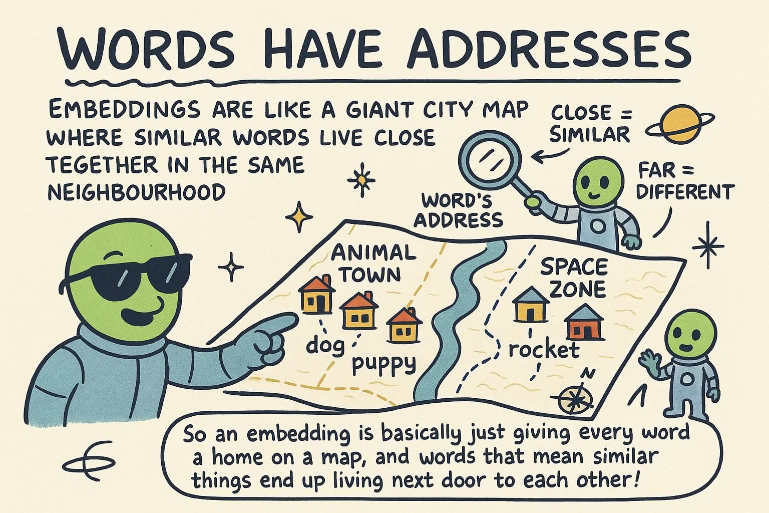
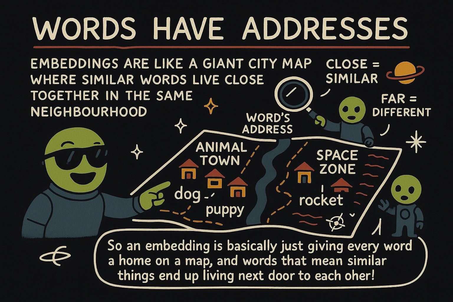
A rough mental picture: imagine every piece of text placed as a dot in space, where things that mean similar things are near each other. "Dog" and "puppy" land in the same neighbourhood. "Stapler" is across town. Real embeddings use hundreds or thousands of dimensions rather than the two or three you can picture, but the intuition holds: closeness means similarity.

Where do those numbers come from, and why do they line up with meaning? An embedding model is a close cousin of the predicting model from How LLMs work, trained on a huge amount of text. To get good at its task it had to learn which words and ideas appear in similar contexts, the old observation that you know a word by the company it keeps.

"Dog" and "puppy" turn up in the same kinds of sentences, so the model learned to represent them similarly. "Stapler" keeps different company, so it sits elsewhere. The hundreds of numbers are learned directions of meaning, each capturing some axis of how text varies, none of them labelled in a way a human would read. You never decode the numbers, you only measure how close two vectors are.

JunoText as vectors An embedding is a list of numbers, a vector, that represents the meaning of a piece of text, produced by a model trained on huge amounts of text. It learned to place words and ideas that appear in similar contexts near each other, so similar meanings get similar vectors. You never read the numbers, you only measure how close two of them are, and closeness reflects meaning.

You want search that matches on meaning instead of spelling, so "get my money back" finds a line about refunds. The move is to turn each piece of text into a vector, a fixed-length list of numbers where similar meanings sit close together. An embedding model reads the text and emits that vector, and the whole point is that distance between vectors stands in for similarity of meaning.

The vector has a set length, its dimension, often a few hundred to a couple thousand numbers. Every text you embed with the same model comes out the same length, which is what lets you compare any two of them. Those dimensions are learned directions of meaning, not human-labelled categories, so you do not read dimension 47 as "formality". You treat the vector as one opaque point and measure distances.

Before you embed anything real, there is a step that decides whether the whole thing works: chunking. You rarely embed a whole document as one vector, because one vector for a 20-page manual blurs every topic in it into a single average point that matches nothing well. Instead you split the document into chunks, passages of roughly a paragraph to a page, and embed each chunk on its own. Embed chunks, not whole documents, so each vector carries one focused idea.

Chunk size is a real trade-off you set deliberately. Chunks that are too large average several ideas together and retrieve loosely. Chunks that are too small lose the surrounding context that made a sentence meaningful. A common starting point is a few hundred tokens per chunk with a small overlap between neighbours, so a sentence split across a boundary still appears whole in one of them, then you adjust based on what your retrieval actually returns.

JunoText as vectors An embedding turns text into a fixed-length vector where distance stands in for similarity of meaning, and every vector from the same model shares a length so you can compare them. The dimensions are learned directions, not labels, so treat the vector as one opaque point. Here is the move that matters most: chunk your documents into paragraph-sized passages and embed each chunk, because one vector for a whole document averages everything into mush.

Search that matches on meaning rests on one idea: map text into a vector space (a fixed-dimensional coordinate space where each point is a list of numbers) such that semantic similarity becomes geometric proximity. An embedding model is the map: it reads text and returns a vector.

Everything you build on top, indexing, retrieval, ranking, is geometry over those vectors. Get the mapping wrong and nothing downstream recovers it.

The first design lever is what you embed, and that is chunking: splitting source documents into passages before embedding rather than embedding whole files. The reason is that an embedding is a lossy compression of its input into one point, so the more distinct ideas a chunk contains, the more they average into a vague centroid that retrieves nothing sharply. Right-size the chunk to the unit a user will ask about, usually a passage of a few hundred tokens, with a small overlap so a fact straddling a boundary survives in at least one chunk.

Chunking strategy is where retrieval quality is won or lost, more than the model choice:

• Fixed-size windows are cheap, but they cut sentences mid-thought.
• Structure-aware splitting (on headings, paragraphs, or code blocks) keeps each chunk coherent and tends to retrieve better, at the cost of a more involved pipeline.

Whatever you pick, store the chunk's source and position alongside its vector, because at retrieval time you need to point back to where a fact came from, and a bare vector cannot tell you.

One more property to internalise: embedding dimensions are not interpretable axes, so you cannot debug retrieval by reading a vector. You debug embeddings by inspecting what they retrieve, never by reading the numbers. When a query pulls the wrong chunk, the fix is in the chunking, the model, or the query, examined through retrieved results, not through the coordinates themselves.

JunoText as vectors An embedding model maps text into a vector space where semantic similarity becomes geometric distance, and every later step is geometry over those points. Chunking is the lever that decides retrieval quality: size chunks to the unit a user asks about, split on structure where you can, and store each chunk's source and position next to its vector so you can trace a fact back. You cannot read a vector to debug it, so when retrieval goes sideways, inspect what came back, not the numbers.

Generating an embedding

You ask an embedding model for the vector, much like a normal model call but with a different endpoint and a different model.

from openai import OpenAI

client = OpenAI()

EMBED_MODEL = "text-embedding-3-small"  # swap point for the embedding model

def embed(text):
    response = client.embeddings.create(model=EMBED_MODEL, input=text)
    return response.data[0].embedding  # a list of numbers

vector = embed("a small playful dog")
print(len(vector))  # e.g. 1536 numbers

The result is a list of numbers. One rule matters above the rest: always compare embeddings made by the same model. Vectors from different models live in different spaces and are not comparable, like measurements in different units. Mixing models gives nonsense scores, every time.

And like every model call, you are billed by tokens, so embedding a large document collection has a cost worth estimating up front before you run it across thousands of documents.

JunoGenerating an embedding You generate an embedding by calling an embedding model, which hands back a list of numbers for your text. Always compare vectors made by the same model, because different models produce vectors that are not comparable, like centimetres against inches. Embedding is billed by tokens, so a large collection has a real cost worth checking first.

The call itself is a different endpoint with the same shape as a chat call: you send text, you get a vector back.

from openai import OpenAI

client = OpenAI()

EMBED_MODEL = "text-embedding-3-small"

def embed_batch(texts):
    # send many texts in one request, get one vector per text back
    response = client.embeddings.create(model=EMBED_MODEL, input=texts)
    return [item.embedding for item in response.data]

chunks = ["a small playful dog", "a young dog", "an office supply"]
vectors = embed_batch(chunks)  # one vector per chunk, same order in

The shape varies by provider, but the request-and-response idea is the same everywhere. Two practical points beyond the basic call. First, embed in batches: most endpoints take a list of texts in a single request and return one vector each, which is faster and cheaper than one call per chunk because you pay less request overhead and hit rate limits less. When you index a large corpus, batching is what keeps the cost and the wall-clock time sane.

Second, the same-model rule has a partner: model and dimension are a choice, not a default. Bigger embedding models with more dimensions capture finer distinctions but cost more to compute, store, and compare. Pick the smallest model and dimension that still separates your data.

Some models even let you request a shorter vector to trade a little accuracy for cheaper storage and faster search. Whatever you choose becomes a contract: change the model later and every stored vector has to be regenerated.

JunoGenerating an embedding Embedding is one request that takes text and returns a vector, and the same shape works across providers. Batch your texts into a single call when you can, because it cuts request overhead and rate-limit pressure across a large corpus. Model and dimension are a real choice: pick the smallest that still separates your data, and remember the model becomes a contract, since changing it means re-embedding everything you stored.

The API surface is small. You send text, you get a float vector, and the interesting decisions sit around that call rather than in it.

from openai import OpenAI

client = OpenAI()

EMBED_MODEL = "text-embedding-3-small"

def embed_batch(texts):
    # one request, many vectors back, in input order
    response = client.embeddings.create(model=EMBED_MODEL, input=texts)
    return [item.embedding for item in response.data]

The request and response shape varies by provider, but every embedding endpoint is this same batch-in, vectors-out contract. Batching is not a nicety at scale, it is the difference between an index job that finishes and one that throttles all afternoon: each request carries fixed overhead and counts against a rate limit, so amortise both by sending large batches, then back off and retry on the partial failures a big job will hit.

Model and dimension are an architectural commitment with a long tail. Higher-dimensional vectors store more distinction but cost more on every axis that matters in production: storage per vector, memory in the index, and time per comparison, all scale with dimension. Some models support Matryoshka embeddings (vectors you can truncate to a shorter length and still use), which let you keep full vectors for accuracy and serve a truncated prefix for cheap first-pass search. Worth it when your corpus is large enough that storage and query latency, not model quality, are the binding constraint.

The commitment that bites later is versioning. A stored embedding is tied to one exact model version forever.

Vectors from two model versions are not comparable, so you cannot embed a new query with a newer model and compare it against an index built on the old one. The result is silent: scores look plausible and rankings are wrong. Treat the model version as part of your index's schema, store it alongside the vectors, and plan re-embedding as a migration, covered in the freshness discussion later in this chapter.

JunoGenerating an embedding The embedding call is a batch-in, vectors-out contract that varies in shape by provider but not in idea, and batching with retry is what makes a large index job finish instead of throttle. Model and dimension scale storage, memory, and query latency, so reach for truncatable vectors when scale, not quality, is the constraint. The version is a forever commitment: vectors from different model versions silently fail to compare, so store the version in your schema and treat re-embedding as a planned migration.

Measuring similarity

To find how related two pieces of text are, you measure how close their vectors are. The standard measure is cosine similarity, which returns a number from -1 to 1: closer to 1 means more similar, near 0 means unrelated. You do not need the math behind it to use it. Think of it as comparing the direction two vectors point.

Direction is what carries the meaning here, which is why cosine compares angle rather than raw distance. Two texts about refunds point the same way whether one is a short phrase or a long paragraph.

import math

def cosine_similarity(a, b):
    dot = sum(x * y for x, y in zip(a, b))
    mag_a = math.sqrt(sum(x * x for x in a))
    mag_b = math.sqrt(sum(x * x for x in b))
    return dot / (mag_a * mag_b)

dog = embed("a small playful dog")
puppy = embed("a young dog")
stapler = embed("an office supply for binding paper")

print(cosine_similarity(dog, puppy))    # higher, the two are close in meaning
print(cosine_similarity(dog, stapler))  # lower, the two are unrelated

The numbers confirm the intuition: dog and puppy score higher, dog and stapler score lower. Comparing a query's vector against stored vectors is the heart of semantic search. That one function is the move the rest of the chapter builds on.

JunoMeasuring similarity Cosine similarity scores how close two vectors are, from -1 to 1, where closer to 1 means more similar. You can use it without the math, it compares the direction two vectors point, which is why a short phrase and a long paragraph about the same thing still match. Comparing a query's vector against stored vectors is the core move of semantic search.

You have vectors, now you need a number that says how close two of them are. The standard is cosine similarity: it measures the angle between two vectors, ignoring their length, and returns a value from -1 to 1 where higher means more alike. Angle, not distance, is what you want, because a long passage and a short phrase on the same topic should score as similar even though their vectors have different magnitudes.

def dot(a, b):
    return sum(x * y for x, y in zip(a, b))

# if vectors are normalized to length 1, cosine similarity equals their dot product
score = dot(query_vector, doc_vector)  # no division needed

Here is the move that pays off at scale: normalize your vectors to length 1 when you store them. Once every vector has the same length, the division in cosine similarity disappears and the score becomes a plain dot product, which is one multiply-and-add per dimension and much faster to run across a large set. Normalize once at storage, then compare with a dot product. Many embedding models return already-normalized vectors, but do not assume it, check.

The other shift from the toy example: you rarely want the single closest match. You want top-k retrieval, the k highest-scoring results, usually three to ten. One vector can be a near-miss while the second and third together hold the answer, and returning a small set gives the next stage room to work. Returning only the top one throws away context you will wish you had kept.

JunoMeasuring similarity Cosine similarity compares the angle between two vectors from -1 to 1, ignoring length, so a short phrase and a long passage on the same topic still match. Normalize your vectors to length 1 at storage time and the comparison collapses to a fast dot product, which adds up across a big set. And retrieve top-k, three to ten results, not the single best, because the answer is often spread across the first few.

You need a similarity metric, and cosine similarity (the cosine of the angle between two vectors, ranging -1 to 1) is the default because it ignores magnitude, so document length does not swamp topic. That choice has a performance consequence worth designing around: cosine over raw vectors costs a dot product plus two magnitude computations per comparison, and you pay it for every vector in the index on every query.

import numpy as np

# normalize at write time, once per vector
def normalize(v):
    v = np.asarray(v, dtype=np.float32)
    return v / np.linalg.norm(v)

# at query time, cosine over normalized vectors is a single matrix-vector product
def search(query_vec, matrix):
    return matrix @ query_vec  # one score per row, vectorized

The optimisation is to normalize every vector to unit length at write time, which makes cosine similarity identical to a dot product and lets you score the whole corpus as one matrix-vector multiply instead of a Python loop. Normalize at write time and similarity is a dot product over the whole index at once. This is the brute-force baseline: exact, direct, and linear in corpus size, which is fine up to roughly the low hundreds of thousands of vectors and falls over above that, the cue to move to an approximate index covered later.

Two production realities the toy metric hides. First, you almost never want the argmax, you want top-k with a score threshold, because the gap between the first and second result tells you how confident the match is, and a top result that still scores low means nothing in your corpus actually answered the query. Return that as "no good match" rather than handing back the least-bad row. Second, cosine similarity is relative, not absolute: a score of 0.4 is meaningful only against the distribution of scores your corpus and model produce, so calibrate thresholds empirically per index rather than copying a magic number from a blog post.

JunoMeasuring similarity Cosine similarity ignores magnitude so length does not drown topic, but brute-force cosine is linear in corpus size and only holds to the low hundreds of thousands of vectors before you need an approximate index. Normalize at write time and the metric becomes a dot product you can run as one matrix-vector multiply over the whole corpus. Retrieve top-k with a threshold, treat a low top score as no match rather than the least-bad row, and calibrate that threshold per index because the numbers are relative, not absolute.

Semantic search

Put the pieces together and you can search by meaning instead of keywords. Embed your documents once and store the vectors. When a query comes in, embed it too, then return the documents whose vectors are closest.

docs = [
    "Reset your password from the account settings page.",
    "Our refund policy allows returns within 30 days.",
    "Contact support by email for billing questions.",
]

# embed every document once, up front
index = [{"text": text, "vector": embed(text)} for text in docs]

def search(query):
    query_vector = embed(query)
    scored = [{"text": item["text"], "score": cosine_similarity(query_vector, item["vector"])} for item in index]
    return sorted(scored, key=lambda x: x["score"], reverse=True)[0]  # the closest match

print(search("how do I get my money back?"))
# returns the refund-policy line, even though it shares no keywords with the query

The query "how do I get my money back?" finds the refund line despite sharing no important words with it. Semantic search matches on meaning, not spelling. Keyword search would have missed it entirely, because the query and the document have no important words in common.

The shape is always the same: embed once and keep the vectors, embed the query at request time, score, sort, return the closest. That is the semantic search loop, and you will reuse it for the rest of this handbook.

JunoSemantic search Semantic search embeds your documents once and stores the vectors, then embeds each incoming query and returns the closest documents by cosine similarity. It matches on meaning, so "get my money back" finds a "refund policy" line that shares no keywords. That meaning-based matching is the thing keyword search cannot do.

The toy version stores vectors in a Python list and scores every one on each query. That works for a demo and breaks the moment your corpus grows, because a linear scan re-runs the full comparison over every vector for every query, and you are also rebuilding the index in memory on every restart.

The fix is a vector database: a store built to hold vectors and answer "find the nearest k to this query vector" quickly and from disk. Instead of your own list and loop, you write vectors in once and the database handles the search, persistence, and updating individual entries.

# shape varies by vector DB, but the pattern is the same everywhere
index.upsert([
    {"id": "doc-1", "vector": embed(chunk), "metadata": {"source": "faq.md", "section": "refunds"}}
    for chunk in chunks
])

results = index.query(vector=embed(user_question), top_k=5)  # nearest 5, not only 1

Two things the database gives you that the list does not:

• It returns top-k results in one call, the nearest several rather than a single best, which is what you actually feed the next stage.
• It stores metadata next to each vector, the source file, section, and timestamp, so a result can point back to where it came from and you can filter by it.

Store vectors in a vector DB, not a Python list, the moment you have real data. The list is for learning the mechanism, not for running it.

JunoSemantic search Semantic search is embed-once, store, embed the query, return the nearest, but a Python list and a loop only survive a demo, because scanning every vector per query and rebuilding on restart does not scale. Move to a vector database the moment you have real data: it does fast top-k search from disk and stores metadata next to each vector so results point back to their source. The list teaches the mechanism, the database runs it.

The reference loop, embed once, store, embed the query, score, sort, return, is correct and does not survive contact with scale. A brute-force scan is linear in corpus size per query, so at a million vectors and any real query rate you are spending a CPU-second per search you do not have. Everything in production search is about not comparing the query against every vector.

That is what approximate nearest neighbor search buys you (ANN: algorithms that find the closest vectors fast by accepting a small chance of missing a true nearest one). Two families dominate:

• HNSW (Hierarchical Navigable Small World) builds a layered graph of vectors and walks it from coarse to fine, giving low query latency at the cost of high memory.
• IVF (inverted file) clusters vectors and searches only the nearest clusters, using less memory but needing its cluster centers retrained as data shifts.

Above a few hundred thousand vectors, ANN is not optional, it is the index. The trade-off you are tuning is recall (the fraction of true nearest neighbors the index actually returns) against latency and memory: push recall toward 1.0 and queries slow down, relax it and you silently miss relevant chunks.

The failure mode the toy loop hides entirely is freshness. An index is a snapshot, so when a source document changes, its stored vector is now stale and keeps getting retrieved as if current. You need a re-embedding pipeline keyed on document change: detect the edit, re-chunk and re-embed that document, and upsert the new vectors while deleting the old ones, ideally tracked by a content hash so you re-embed only what actually changed rather than the whole corpus on every edit. Stale vectors are the quiet way a retrieval system starts lying.

The last gap is exact match. Vector search is built to miss it: a query for order A-10293 or an error code embeds to a fuzzy region and may not surface the one document that contains that string. Hybrid search runs keyword search (which nails exact tokens) and vector search (which nails meaning) together and merges the rankings, so identifiers, names, and rare terms are not lost to semantic blur. Reach for it whenever your corpus contains things users will type exactly.

JunoSemantic search A brute-force scan dies at scale, so above a few hundred thousand vectors you run approximate nearest neighbor, HNSW for low latency at high memory or IVF for the reverse, and you tune recall against latency knowing higher recall costs speed. Build a re-embedding pipeline keyed on document change with a content hash, because an index is a snapshot and stale vectors retrieve as if current. And add hybrid keyword-plus-vector search whenever users type exact strings like order numbers, since pure vector search blurs right past them.

What embeddings are not for

Embeddings are a similarity tool, not a thinking tool. A few limits to keep in mind so you reach for the right tool:

• They do not do exact matching. To find an exact order number or an error code, plain keyword or database search is better.
• They do not reason. They tell you two things are related, not why, and not whether one logically follows from the other.
• They go stale. If your documents change, you must re-embed them, or your search points at old content.

Embeddings find what is related, they do not judge what is true or current. Each of these gaps has a better tool, and knowing which to use is half the skill.

JunoWhat embeddings are not for Embeddings measure similarity, they do not reason and they do not do exact matching. For an exact order number or error code, use keyword or database search instead. And when your documents change, re-embed them, or your search will point at stale content.

The trap with a tool that works this well is reaching for it everywhere. Three limits mark where to stop and pick something else.

Exact matching is the first. Embeddings map an order ID or an error code into the same fuzzy semantic space as everything else, so A-10293 lands near other order-shaped strings, not exactly on itself. For identifiers, codes, and any value a user types literally, keyword or database search is the right tool, and hybrid search (keyword and vector search run together) is how you get both at once.

Reasoning is the second. Similarity is not inference: two chunks scoring high means they are about related things, not that one answers a question or logically follows from the other. The reasoning happens in the model you feed the retrieved chunks to, not in the retrieval. Retrieval finds candidates, the model does the thinking.

Freshness is the third and the one that bites quietly. Your index is a snapshot from whenever you embedded it, so edited documents keep returning their old wording until you re-embed. Treat re-embedding on change as part of the system, not a thing you do by hand when someone notices the answers went wrong.

JunoWhat embeddings are not for Embeddings are a similarity tool, so they miss exact matches like order IDs, which want keyword search or a hybrid of both, and they do not reason, the model you feed the chunks to does that. The quiet one is freshness: an index is a snapshot, so edited documents keep returning stale wording until you re-embed. Build re-embedding into the system rather than waiting for someone to notice wrong answers.

Knowing where embeddings stop is what keeps a retrieval system reliable, and three boundaries matter in production.

Exact match is a structural blind spot, not a tuning problem. Embeddings compress input toward semantic neighborhoods, so identifiers, codes, SKUs, and rare proper nouns get smeared toward similar-looking strings rather than landing on themselves. Pure vector search will rank a near-miss above the exact hit. The fix is hybrid retrieval that fuses a lexical index (keyword or BM25, a classic term-frequency ranking) with the vector index, so exact tokens are matched exactly while meaning is matched semantically, and you do not gamble an order lookup on geometry.

Drift is the boundary that erodes silently. Embedding drift is the mismatch you get when the model version behind your index changes: vectors from two versions occupy different spaces and are not comparable, so a query embedded with a new model against an index built on the old one returns plausible-looking nonsense. Pin the model version in your index schema, and treat any model upgrade as a full re-embed migration, not a drop-in, because there is no error thrown, only quietly worse results.

Evaluation is the boundary people skip until retrieval is already failing. You cannot eyeball whether retrieval is good, you measure it: hold out a set of queries with known-relevant chunks and score recall@k (did the right chunk land in the top k) and precision (how much of what you returned was relevant). If you are not measuring recall@k, you do not know if retrieval works.

That eval set is also what tells you whether a new chunking strategy, model, or hybrid weighting actually helped, rather than trading one set of failures for another you have not noticed yet. Retrieval quality is the foundation RAG stands on, so it earns a real test, not a vibe check.

JunoWhat embeddings are not for Embeddings have a structural blind spot for exact matches, so fuse a lexical index with the vector one for identifiers and codes rather than trusting geometry. Embedding drift is the silent one: vectors from different model versions do not compare, so pin the version and treat upgrades as a full re-embed. And measure retrieval with recall@k on a held-out set, because you cannot eyeball whether it works, and that eval is also how you tell a real improvement from a lateral move.

In practice

The full flow lives in the search function above: embed a small set of FAQ entries once, then answer queries by meaning. The pattern is the same at any size, only the storage changes as you grow.

In the next chapter you take the closest matches and feed them to a model, so it answers from your documents instead of from memory. That technique is RAG, and it is built directly on what you wrote here.

JunoIn practice Semantic search is the whole flow: embed your documents once, then for each query embed it and return the closest by cosine similarity. Feed those closest matches to a model and it can answer from your documents instead of memory. That is retrieval, the next chapter, built directly on this.

The mechanism is settled: chunk, embed in batches, store in a vector DB, retrieve top-k by similarity. What changes as you go to production is the surrounding plumbing, the re-embedding on change, the metadata you filter on, the model version you pin.

The retrieved chunks are not the end. In the next chapter you feed them to a model as context so it answers from your documents rather than its frozen training. That is RAG, and the quality of its answers is capped by the retrieval you build here.

JunoIn practice The loop is chunk, batch-embed, store in a vector DB, retrieve top-k, and production is the plumbing around it: re-embedding on change, metadata filters, a pinned model version. Those retrieved chunks become context for a model in the next chapter, which is RAG. Its answers are only as good as the retrieval you set up here.

Everything here, chunking, normalization, ANN indexing, hybrid retrieval, freshness, and recall@k evaluation, is the retrieval layer, and it is the part of an AI system that quietly determines whether the answers are any good. The model on top can only reason over what retrieval hands it, so a confident wrong answer is usually a retrieval failure wearing a generation costume.

That is the bridge to the next chapter. RAG is this retrieval layer feeding grounded context into a model, and every failure mode here, stale vectors, missed exact matches, low recall, surfaces there as a wrong answer. Build the retrieval to be measured and fresh, and RAG has something solid to stand on.

JunoIn practice The retrieval layer, chunking through recall@k, is what decides whether the answers are good, because the model only reasons over what retrieval hands it. A confident wrong answer is usually retrieval failing in disguise, so the stale vector or the missed exact match is the real bug. RAG in the next chapter is this layer feeding a model, and it is only as solid as what you build here.